Exploring Chemistry includes discussion of many advanced modeling techniques. One example is Franck-Condon analysis of excited states, which may be used to model fluorescence and emission.

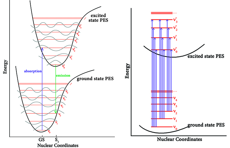
The quantity that is computed in a standard TD-DFT calculation is the energy change for a molecule going from some point on the ground state (GS) potential energy surface—ideally the minimum—to the point on the excited-state (XS) potential energy surface that is at the same geometry as the ground state. This is known as a vertical transition. The transition labeled “absorption” in the left figure above provides an example, with the length of the arrow representing the excitation energy.

In this example, the geometry of the excited state immediately after absorption of a photon is not the minimum on its potential energy surface. Moreover, the vibrational state is not the lowest one either. Because the time scale in which electronic transitions occur is so small compared to nuclear motions, the nuclei are nearly unaffected, and the electric dipole can be considered constant during the transition. For this reason, the geometry of the excited state is initially unchanged from the ground state, and the same is true of its vibrational states. When the molecule transitions to the excited state, it moves to a vibrational state that is instantaneously compatible with its current vibrational state.

These effects are the basis of the Franck-Condon principle which states that a molecule may undergo a transition to a different, higher vibrational level in an excitation to an excited state or a relaxation back to the ground state. The probability of a vibrational transition to a particular vibrational state is proportional to the overlap integral between the initial and final vibrational states. This means that the final vibrational state is the one which closely resembles the initial vibrational state. In qualitative terms, this means that the final vibrational state is the one which most closely resembles the initial vibrational state. In the absorption example in the figure, the molecule transitions from the lowest vibrational state at the ground state geometry to the third vibrational state as it absorbs a photon and enters the first excited state.

Shortly thereafter, the geometry will relax to the minimum on the excited state potential energy surface (labeled “S1” in the diagram). The molecule may then relax back to the ground state, emitting a photon in the process. This process will once again happen essentially instantaneously with respect to nuclear motion, and it may also involve a vibronic transition. The arrow labeled “emission” in the preceding figure provides an example. Note that the Franck-Condon principle applies to both absorption and emission.

This description, while more nuanced than our initial descriptions of excitation, is still a simplification. In reality, a sample present in a spectrometer at room temperature will have molecules with energies distributed among the various vibrational levels as dictated by the Boltzmann distribution formula. Therefore, the actual energy transition observed in the experiment is actually a series of many energy transitions from the various vibrational levels of the ground state to the various vibrational levels of the excited state. The strength of each individual transition will depend on the population of that state (which is temperature dependent) and the overlap between the ground and excited vibrational wave functions for that transition.

The figure on the right above captures some of this complexity. This figure shows the potential transitions for the four lowest vibrational states, considering only the same vibrational states for the excited state. The effect on the observed spectrum is to give the peak associated with an electronic transition additional structure in the form of sub-peaks: many lines instead of only a single absorption line. The Franck-Condon analysis features in Gaussian can be used to model this phenomenon.